The Art of Scaling RL Compute for LLMs
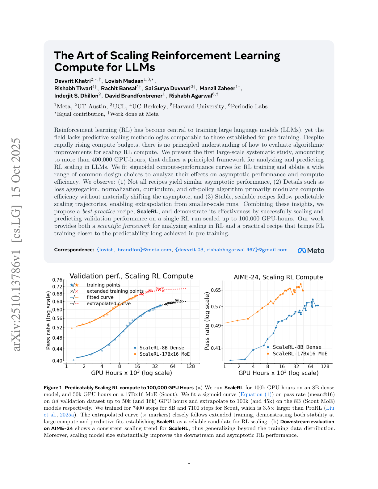
A 400k+ GPU-hour study introduces a simple, predictive way to scale RL for LLMs. The authors fit a sigmoidal compute→performance curve that lets you extrapolate from small runs and propose ScaleRL, a stable recipe validated up to 100k GPU-hours on an 8B dense model and a 17B×16 MoE.
Ask this paper
Predictive scaling law you can actually use: Model pass-rate vs log(compute) follows a saturating sigmoid with three knobs: A (asymptotic ceiling), B (compute efficiency), Cmid (midpoint). Fit after ~1.5k GPU-hours on a 1k-prompt holdout, and you can forecast larger budgets. This matched extended training in practice, including the 100k GPU-hour run and MoE scaling.
ScaleRL recipe that held up under leave-one-out: PipelineRL with k=8, CISPO loss (truncated IS REINFORCE), prompt-level loss averaging, batch-level advantage norm, FP32 logits at the LM head, zero-variance prompt filtering, No-Positive-Resampling curriculum, and forced interruptions to cap thinking length. LOO ablations to 16k GPU-hours show ScaleRL as the most efficient while retaining similar or better asymptotes.
What actually moves the ceiling vs just speed: Not all popular RL recipes converge to the same A. Loss choice and precision at logits lift the ceiling, while aggregation, normalization, curriculum, and off-policy details mostly tune B. CISPO/GSPO > DAPO on asymptote; FP32 logits gave a big jump (A≈0.52→0.61).
Scaling axes that paid off: • Longer generation budgets (to 32k) raise the asymptote at the cost of early efficiency. • Bigger global batches improve asymptote and downstream generalization, avoiding small-batch stagnation. • Larger models (MoE) deliver much higher asymptotic RL performance with less compute than the 8B dense. • More generations per prompt at fixed total batch size is second-order.
Operator notes for stable long runs: Fit curves on a held-out 1k-prompt set with mean@16 generations, watch truncation rates as an instability signal, prefer interruptions over length penalties for length control, and plan early small-budget ablations to choose methods that scale by A first, then tune B.